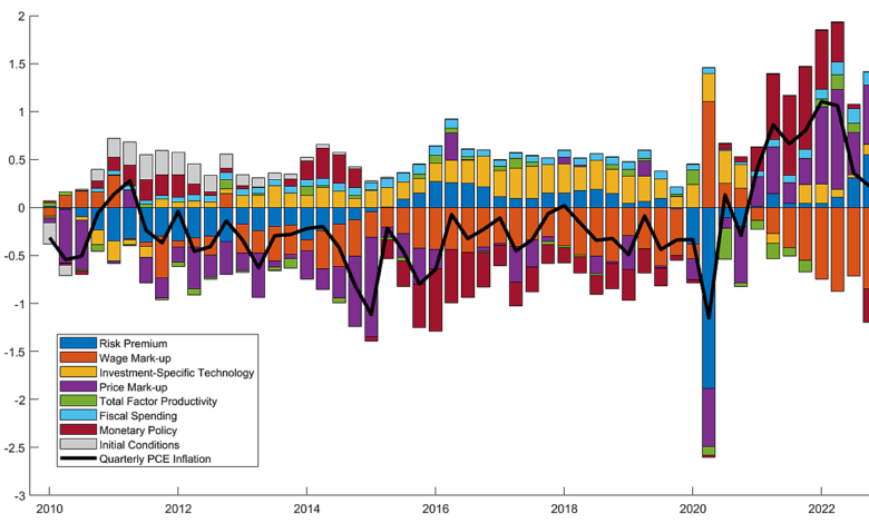
Fiscal Spending Contributed to Post‐COVID‐19 Inflation

A CMFA article, published a few months ago, used a standard empirical macroeconomic model to bridge the two varying explanations for the post‐COVID‐19 inflation spike—supply problems and poor monetary policy. The use of a standard model showed that both factors played a role in causing inflation. The Joint Economic Committee recently released the 2023 Joint Economic Report (“JER”); a section on the fiscal causes of inflation references our prior CMFA article (see Box 1–3, pp. 181–183). It critiques our finding that fiscal spending had a minor deflationary effect because economic theory suggests that government handouts raise demand, thereby increasing prices. While the purpose of that CMFA article was simply to bridge the inflation explanations provided by Bernanke‐Blanchard and Jason Furman at a Brookings event, not to specifically measure fiscal effects on inflation,[1] the JER’s point—which is essentially about an idea known as Ricardian equivalence—is well taken.
Ricardian equivalence is a well‐known and longstanding facet of economic models that include perfectly rational and forward‐looking consumers. Such consumers would know that any current government spending would necessarily be financed with tax increases in the future; consequently, they would save any current fiscal stimulus for future expenses and government spending would have no discernable effect on model variables.
The Smets and Wouters (2007) (SW) model, used in the CMFA article, contains such agents and in turn exhibits Ricardian equivalence. Therefore, to more accurately study the effects of fiscal stimulus, a different model such as Gali, Lopez‐Salido, and Valles (2007) (GLV) is more useful. The GLV model assumes that a fraction of consumers does not have access to savings institutions and spends their entire per‐period income on consumption (so called “hand‐to‐mouth” or “non‐Ricardian” consumers). Consequently, fiscal spending can have effects on the real economy since these consumers cannot set aside savings today to account for government budget balances in the future.
This article incorporates GLV‐style non‐Ricardian agents into the SW model to create a medium‐scale model that is more useful for fiscal spending analysis. This approach has the dual beneficiary effects of relying on the features of a standard benchmark macro model while also exhibiting the true effects of fiscal spending. The model is estimated to fit key U.S. macro time series data using a Bayesian MCMC algorithm. In line with empirical estimates, the share of non‐Ricardian agents is fixed at 35 percent of U.S. consumers. While the in‐depth details on the model are not included in this blog post, interested readers may find a full description of the model equations and empirical method here.
Figure 1 shows the same inflation breakdown from 2010 to 2022 into the same constituent shocks as our previous article. Note that price markup shocks, capturing supply factors in the goods market, as well as monetary policy, remain the key determinants of post‐COVID‐19 inflation. However, the effect of fiscal spending flips and now has a positive inflationary effect. The effect is not as strong as supply shocks or monetary policy, but nonetheless bridges the distortion between the negative effect of fiscal spending from the SW model and the Ricardian equivalence critique of the JER.
Not only do these results corroborate the JER critique, but they also demonstrate a key flaw in President Biden’s incorrectly named Inflation Reduction Act and its effect of the macroeconomy. While much of the conversation has surrounded the role of the Fed in allowing inflation to spiral, this is a good reminder that both fiscal and monetary authorities must act responsibly to keep prices stable.
For more information on the model, empirical methodology, and posterior distribution please click here.
[1] It is also important to accurately interpret the findings from such decompositions. For instance, an important reason why monetary policy was so loose in this period was to accommodate the increased fiscal spending (see this IMF article).


